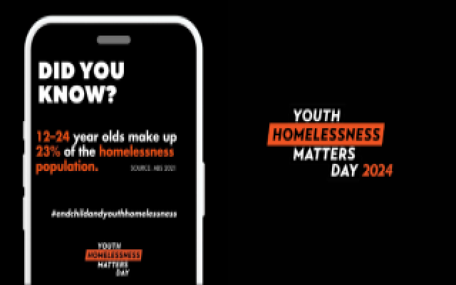
Recognising Youth Homelessness Matters Day 2024
Today is Youth Homelessness Matters Day
Continue reading Recognising Youth Homelessness Matters Day 2024
Today is Youth Homelessness Matters Day
Continue reading Recognising Youth Homelessness Matters Day 2024

Australians in need of family, domestic and sexual violence support now have an additional avenue for receiving assistance, with the official launch today of a new, on-demand video counselling service through 1800RESPECT.
Continue reading 1800RESPECT is increasing its options for victim-survivors seeking support
Learn more about our first step toward future improvements to the NDIS.
Continue reading NDIS Reforms – ‘Getting the NDIS Back on Track’ Bill webinars
Impact Investing Australia and Social Enterprise Australia working together for SEDI
Continue reading SEDI Grants Administrator and Education and Mentoring Coordinator announced
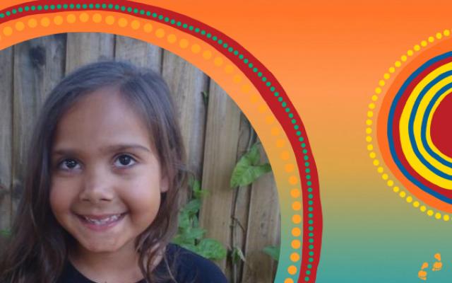
Read the new report of findings and recommendations to support better outcomes for Aboriginal and Torres Strait Islander primary school children.
Continue reading Launch of the Footprints in Time: the Longitudinal Study of Indigenous Children (LSIC) Primary School Report

Join an online webinar for information about the National Disability Insurance Scheme Amendment (Getting the NDIS Back on Track No. 1) Bill.
Continue reading Getting the NDIS Back on Track Bill: Online webinars

Search the DSS Grants Service Directory
DSS grants are now advertised on the Community Grants Hub website.

Opening soon

Opening soon
Closing date: 31 May 2024

Closing date: 30 April 2024
Closing date: 28 April 2024
Closing date: 13 May 2024